Willington Rentería

Como se sabe la relación entre Salinidad, Temperatura y Densidad debe resolverse a través de la Ecuación de Estado. Existe una librería (seawater.gibbs) la misma que puede encontrarse en:  https://pypi.python.org/pypi/gsw.

A continación su aplicación para la resolución de un problema típico en oceanografía física:

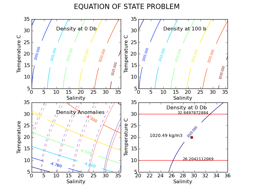
«Make a contour plot of density given a range of salinity from 0 to 36, and temperature from 5 to 35 at zero pressure (i.e., the surface). How do the contours change if the pressure were 100 bar (i.e., 1000 m depth). Plot the anomalies in the density between these two depths, that is the differences in the density at these two depths that are not just changes in the mean density of water between a reference water mass. Use water at 10 deg C and 30 psu as a reference. Find the salinity of water with a density of 1020 kg m−3 at 10_C and at 30_C and zero pressure. What is the density of the water that results from mixing equal parts of these two water masses?»

El código para resolver este problema es el siguiente:

import matplotlib
from numpy import *
import seawater.gibbs as gsw

x = linspace(0,36,50)
y = linspace(5,35,50)
(X,Y) = meshgrid(x,y)

#Density at Zero pressure
do = gsw.rho(X, Y,0)
plt.subplot(2,2,1)
c = plt.contour(X,Y,do)
lx = plt.xlabel("Salinity")
ly = plt.ylabel("Temperature C")
plt.suptitle('EQUATION OF STATE PROBLEM', fontsize=16)
plt.text(10,30,'Density at 0 Db')
plt.clabel(c,inline=1, fontsize=7)

##Density at 100 bar== 1000db[1 dbar = 0.1 bar]
dz = gsw.rho(X, Y,1000)
#dz=dens(X,Y,1000)
plt.subplot(2,2,2)
cz = plt.contour(X,Y,dz)
lx = plt.xlabel("Salinity")
ly = plt.ylabel("Temperature C")
plt.text(10,30,'Density at 100 b')
plt.clabel(cz,inline=1, fontsize=7)
##Density difference
#dr=dz-do
dr=gsw.rho(30,10,0)
dpo=do-dr
dpz=dz-dr
dan=dpo-dpz
plt.subplot(2,2,3)
cr = plt.contour(X,Y,dpo,linewidths=0.5,colors='blue')
ca = plt.contour(X,Y,dpz,linewidths=0.5,colors='red')
ano= plt.contour(X,Y,dan)
lx = plt.xlabel("Salinity")
ly = plt.ylabel("Temperature")
plt.text(10,30,'Density Anomalies')
plt.clabel(ano,inline=1, fontsize=9)

##The final value
a = linspace(20,36,100)
b = linspace(5,35,100)
(A,B) = meshgrid(a,b)
#dm = gsw.rho(A, B, 0)
dm=gsw.rho(A,B,0)
plt.subplot(2,2,4)
level=[1020]
cr = plt.contour(A,B,dm,level)
l = plt.axhline(y=10,color='r')
l = plt.axhline(y=30,color='r')
lx = plt.xlabel("Salinity")
ly = plt.ylabel("Temperature C")
plt.text(25,32,'Density at 0 Db')
plt.clabel(cr,inline=1, fontsize=7)
#looking the values of Salinity
d10=gsw.rho(a,10,0)
d30=gsw.rho(a,30,0)
t10=interp(1020,d10,a)
t30=interp(1020,d30,a)
plt.plot(t10,10,'r+',t30,30,'r+')
#mixing point
Temp=20
Sal=(t30+t10)*0.5
Mix=gsw.rho(Sal,Temp,0)
plt.plot(Sal,Temp,'ro')
plt.text(28,10,t10,fontsize=9)
plt.text(27,30,t30,fontsize=9)
plt.text(22,Temp,'1020.49 kg/m3',fontsize=10)
plt.show()

El resultado es el siguiente: